Tutorials: QEpy

QEpy SCF density update animation — Iterative SCF: QEpy updates the electron density step by step from Python.

Run QEpy as QE (command line)

QEpy can replace standard QE executables. List supported packages:

python -m qepy -h

Options ending in .x mirror QE executables; options ending in .py are QEpy-specific tools.

Serial pw.x equivalent

python -m qepy --pw.x -i qe.in

MPI parallel (OpenMPI / Intel MPI)

mpirun -n 4 python -m qepy --pw.x -i qe.in

QEpy-specific example: analyze and convert pw.x output:

python -m qepy --pw2pp.py -h

HPC clusters (SLURM): on some systems (e.g. Rutgers Amarel) plain mpirun may fail. Use the site-recommended MPI launcher: often srun --mpi=pmi2 -n N python -m qepy .... Check your cluster documentation.

Use QEpy in Python code

The Driver class is the main entry point. Import qepy before mpi4py to avoid FFT allocation errors (see FAQ).

Serial execution

Pass comm=None (default) for a single-process run:

import qepy
from qepy import Driver

driver = Driver('si.scf.in', comm=None)
driver.scf()
energy = driver.get_energy()
driver.stop()

Parallel execution with mpi4py

Pass an MPI communicator so Python and Fortran share the same process layout. Only rank 0 (driver.is_root) should print or write files unless you gather data explicitly.

import qepy
from mpi4py import MPI
from qepy import Driver

comm = MPI.COMM_WORLD
driver = Driver('si.scf.in', comm=comm)

if driver.is_root:
    print(f"Running on {driver.nproc} MPI ranks")

driver.scf()
if driver.is_root:
    print("Total energy:", driver.get_energy())
driver.stop()

Launch with your MPI runner, e.g.:

# OpenMPI / Intel MPI
mpirun -n 4 python my_script.py

# SLURM (example)
srun --mpi=pmi2 -n 4 python my_script.py

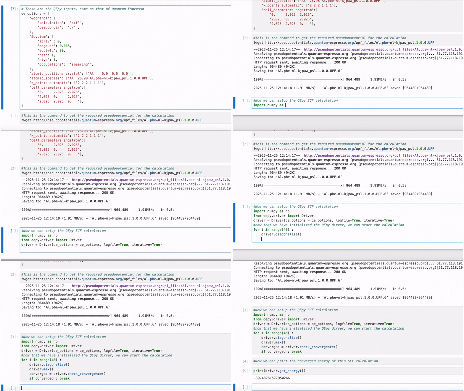
Iterative SCF (step-by-step control)

Set iterative=True to run one SCF iteration at a time: useful for custom mixing, external potentials, or coupling to other models.

driver = Driver('si.scf.in', iterative=True, comm=comm)

while not driver.check_convergence():
    driver.diagonalize()
    driver.mix()
    rho = driver.get_density()
    # inspect or modify rho, set external potentials, etc.

driver.end_scf()
driver.stop()

External potentials & custom XC

# Add an external potential on the real-space grid (Ry units)
v_ext = driver.create_array(kind='rho')
# ... fill v_ext ...
driver.set_external_potential(v_ext)

# Swap XC functional (requires DFTpy integration)
driver.update_exchange_correlation(xc='PBE')

ASE calculator

from ase.build import bulk
from qepy.calculator import QEpyCalculator

atoms = bulk('Si')
calc = QEpyCalculator(inputfile='si.scf.in', comm=comm)
atoms.calc = calc
energy = atoms.get_potential_energy()

Note: ASE uses Å and eV; the Driver uses Bohr and Rydberg. The calculator handles unit conversion.

Jupyter notebooks

Interactive examples live in the QEpy repository under examples/jupyter/. Clone the repo and open them locally, or try the Google Colab notebooks.

Topic	Notebook	What you learn
SCF	`scf/qepy_scf.ipynb`	Basic SCF with the Driver; energy, forces, density.
SCF	`scf/qepy_scf_iterative.ipynb`	Iterative SCF loop with convergence checks.
SCF	`scf/qepy_iterative.ipynb`	Advanced iterative workflow patterns.
SCF	`scf/qepy_qeinput.ipynb`	Build and modify QE input programmatically with `QEInput`.
SCF	`scf/dftpy_mixer.ipynb`	Custom density mixing via DFTpy integration.
Bands / DOS	`band/dos_band_silicon.ipynb`	Band structure and DOS for silicon.
Bands / DOS	`band/dos_band_graphene.ipynb`	Band structure and DOS for graphene.
EOS	`eos/test_eos_vc.ipynb`	Equation of state (volume/consistency tests).
EOS	`eos/test_eos_slow.ipynb`	Slower EOS workflow with detailed output.
Post-processing	`pp/qepy_potentials.ipynb`	Extract Hartree, XC, and local PP potentials.
Post-processing	`pp/qepy_parse_output.ipynb`	Parse QE output files from Python.
Post-processing	`pp/qepy_elf_rdg.ipynb`	Electron localization function (ELF) and reduced density gradient.
Extensions	`ext/dirac_exchange.ipynb`	Custom Dirac exchange functional.
Extensions	`ext/dftpy_xc.ipynb`	User-defined XC via DFTpy.
MD	`nvt/ase_nvt.ipynb`	NVT ab initio MD with ASE + QEpy calculator.
Colab	`colab/qepy_scf.ipynb`	Run QEpy in Google Colaboratory (no local QE build).
Colab	`colab/qepy_colab.ipynb`	Colab setup and environment overview.
Testing	`testing/test_kpoints.ipynb`	K-point convergence workflows.
Testing	`testing/test_ecutwfc.ipynb`	Plane-wave cutoff convergence.
Testing	`testing/test_degauss.ipynb`	Smearing (`degauss`) convergence tests.

Running notebooks with MPI: start Jupyter under an MPI allocation (e.g. srun --mpi=pmi2 -n 4 jupyter notebook) and pass comm=MPI.COMM_WORLD to Driver. For serial exploration, omit comm or use the Colab notebooks.

Video tutorials

QEpy YouTube playlist ↗

These videos span 2021–2025. The current QEpy release (QE 7.2, dev branch) may differ slightly in installation steps, API details, or recommended workflows from what is shown in the older recordings. Use the written tutorials and install guide for up-to-date instructions.

Intro to QEpy June 13, 2021

QEpy for beginners October 10, 2022

Installation of QEpy October 10, 2022

QEpy with ASE October 10, 2022

QEpy on Google Colaboratory October 10, 2022

QEpy on Jupyter Notebooks October 10, 2022

Aniket Mandal, QEpy: Quantum ESPRESSO in Python September 7, 2025

For the full Python API, see The code.